Graphical solution to system of equation(s)
A little in-depth intuition behind solving any system of equations by plotting and finding the solution space.
Introduction
Graphical method comprises of representing the problems (set of functions) on co-ordinate system and identifying the point/region of interest. Before dwelling on how we solve something like linear programming problems with graphical method, first we will have to understand how to solve a system of equations and even before that lets understand what a single equations says.
(1) Solving equation
What if you want to see how the money spend is dependent on the count of apple bought, provided each apple cost 20 bucks. Let’s try to represent this in mathematical form, plot it and try to understand it.
Mathematical Representation:
 single equation with one constraintGraphical Representation:
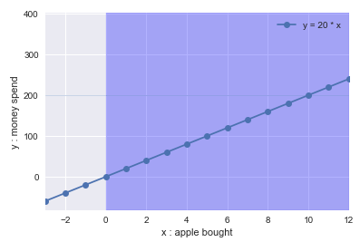 Equation as line, constraint as shaded regionInference:
As evident, the expenditure on apples is directly proportional to the per apple cost (fixed) and apple bought (dynamic). Higher the count of apples, more the money spend. Also, as the numbers of apple bought cannot be negative, so we have a positive constraint on x(shown by shared region). Point to note, the possible value of x and y is determined by the intersection of shaded region and line, which in this case is the positive quadrant.
(2) Solving system of equations
What if you want to find the number of apples to buy, provided you have 200 bucks and each apple cost 20. A simple mental math will give you the answer i.e. 10. But just try to play along for the greater good :)
Mathematical Representation:
 Added one more constraint of maximum spendingGraphical Representation:
 Added constraint of maximum spendingInference:
Just as we added one more constraint of maximum spending being 200, our solution space further reduces. Now our solution should satisfy all three functions (1 equation + 2 constraint) denoted here as the intersection of line and two shaded region. As obvious, with x = 10 we get the best result.
Conclusion
The steps to solve any system of equation is to first transform them into their equivalent mathematical representation. Plot them, determine the solution space and finally select the region/point which maximizes or minimizes the result. This works well for small set of basic equations but becomes tedious with increase in number and complexity. For such cases, classical approaches like linear programming is preferred.