Co-variance: An intuitive explanation!
A comprehensive but simple guide which focus more on the idea behind the formula rather than the math itself — start building the block with expectation, mean, variance to finally understand the large picture i.e. co-variance
 co-variance calculation in all its glory!
Introduction
Contrary to the popular belief, a formula is much more than just mathematical notations. It tries to express an idea, which get hidden under the math and is not evident unless you really look for it. The main problem with this kind of representation (as it usually happens with me), is that after sometime you tend to forget the formula. So, here is my attempt to explain one topic such that it sticks with the audience. Before diving right into it, I will try to explain some prerequisite topics. If you are already familiar with them, feel free to skip. If not, ride along :)
Expectation and Mean
Let’s start with a relatively easier topic which is the one of the basic blocks required to understand co-variance. In probability theory, expectation represents “the expected value of a **discrete random variable*, which is the *probability-weighted average* of all its possible values” *and it is formalized as,
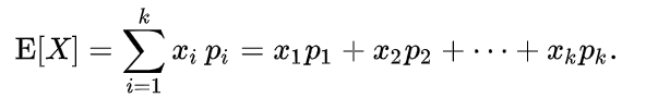 the expectation over all values of ‘X’ and their probabilities ‘p_i’
Here ‘X’ is the variable which can take several shapes — ‘x_i’, where each have it’s own probability ‘p_i’ of occurrence. Notice expected value is a single number representation of all the values a variable can take considering their probabilities. One special case to remember is when all ‘p_i’ are equal i.e. probability of occurrence of all values are equal. In this case, expected value transforms into mean or average. To give an example, suppose a variable which simulates the rolling of an unbiased dice, so the possible values it can take can be 1 to 6. Also the probability of occurrence of any of these numbers will be equal. Coming back to the generalization, the transformation of expectation to mean is showcased below,
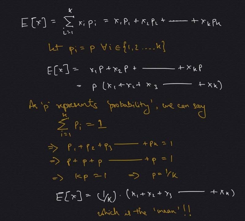 Expectation to mean — how making probability constant makes this possible.
Notice as equal weights are given to all of the values of the variable, the mean is proportional to the values itself, hence it tends to incline towards denser concentration of points. See below a simulation of distribution of points (blue dots) and how change in their position leads to change in the mean (red dot) itself.
 Changing points and chasing mean!
Also be vary of practical simulations, as most of the time they differ from the theoretical simulations. Consider the dice roll example, where we very easily stated that they have equal probability, but a programmed simulation may show some variations. Below, I simulated 10,000 rolls of an unbiased dice. Look at the occurrence distribution of the dice faces.
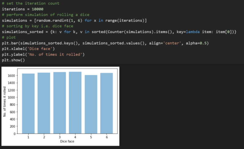 Simulating an unbiased dice roll 10,000 times!
Now compare the theoretical and practical calculation of mean notice there is a difference, even though small, but in practical scenario this will do.
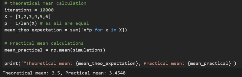 Comparing theoretical and practical mean calculation#### Variance
Observe the following plots, can you find anything common in them?
 Changing points and … wait a sec!?
The answer is — all of them have the same mean! But they look so different, right? And what is so different in all of the them? It seems that they have different ‘spread’ or ‘width’. Variance is basically the measure of this spread or width of the data. In statistics, “variance is the **expectation* of the squared *deviation* of a *random variable* from its *mean*.” *Let’s try to fit this definition to our understanding of expectation,
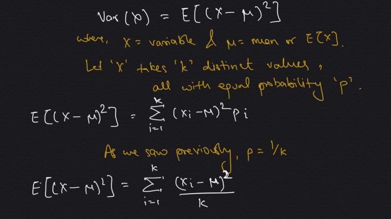 Variance — definition to formula
And just like that we have the formula of variance! Notice first we compute the mean of all the values of ‘X’. Then we find the numerator, which is square of the difference of each value with this mean. The square part is required as we don’t care about the direction of spread, hence we don’t want the spread in opposite directions i.e. with different polarity, to cancel out each other. Some may say, if we square to find the numerator, why not later take a square root? And this idea is exactly represented by standard deviation. So in other words, variance is the square of the standard deviation. With this in mind, let’s look at the same plots as before (now separated and static), but now with variance and standard deviation computed.
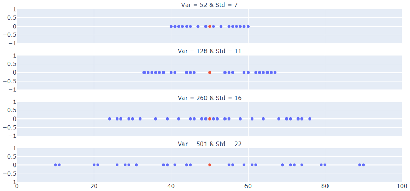 Changing points, static mean but changing variance and standard deviation!
Now we are ready for the main topic but before that there is one more interesting derivation of variance. This isn’t required to understand co-variance but curious readers may want to see it anyways. It represents an idea that, *“variance of a variable is expectation of the squared variable minus the square of the expectation itself”. *It is derived below,
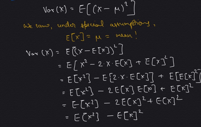 Just another interesting derivation of variance!
While we are at it, let’s compute the variance of the dice roll simulation from before. Also let’s compute the same variance in three different ways, one representing lazy python way and the remaining two representing the formulas we discussed.
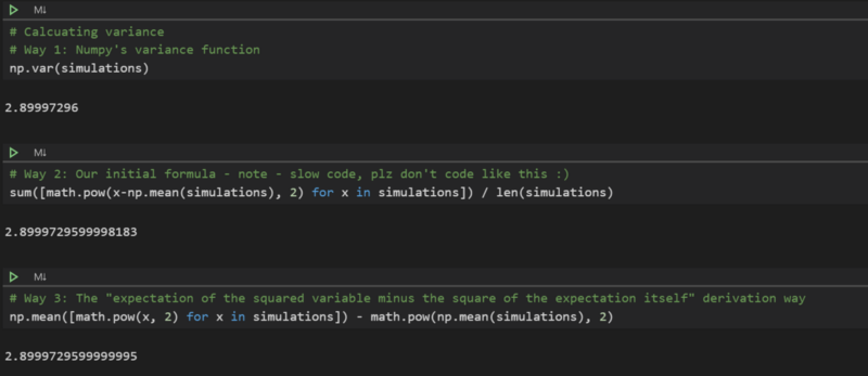 Computing variance in python — sorry for my pythonic one liner codes :)
Note that the variance is same to a certain decimal value, the small difference there is due to the floating point errors. Also, in Python prefer the way 1, I have coded way 2 and way 3, just to showcase the formulas we discussed.
Co-variance
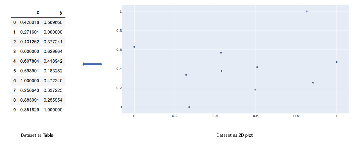
Till now we have been looking at only one variable at a time i.e. our data was 1D or 1-dimensional. Co-variance is defined for higher dimensional data. So as the name suggests, instead of just one variable, it considers multiple (exactly 2) variables and compute variance. Before going further, let’s discuss the data first. When I say 2D, I mean each instance of data is represented by two numbers. And in basic planar geometry, we know two numbers can be associated with a point, hence each instance is represented by a single point. A sample data with 10 instances and their visualization on a 2D plane is shown below,
 Now back to it, more formally co-variance is “a measure of the joint variability of two **random variables*”. *The idea is if both variables follow same increasing behavior we have high co-variance. By this I mean, if one variable increases so does the other. In all of the other cases, like where one increases (or decreases) and the other decreases (or increases), we will have negative co-variance. As its a extension of variance, we can express co-variance formula from variance formula as follows,
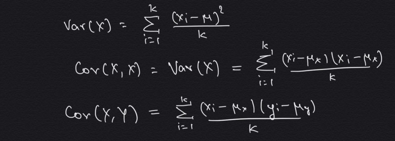 Variance to co-variance
Please note the subtle second line, which says that co-variance of same variable is equal to variance of the variable. And later all we did was to replace the ‘x’ related term from the second portion of numerator with ‘y’, and we have the co-variance formula! Also note that ‘ux’ and ‘uy’ are the mean of variable ‘X’ and ‘Y’ respectively.
One interesting intuition emerges if we look closely at the numerator. But to generalize this, suppose we computed the mean of both variables (‘ux’ and ‘uy’) and took any one point (‘x_i’ and ‘y_i’) from dateset and plotted both of them as points in a 2D plane. Then we can form a rectangle with these two points being at the exact opposite positions. Going in this direction leads to,
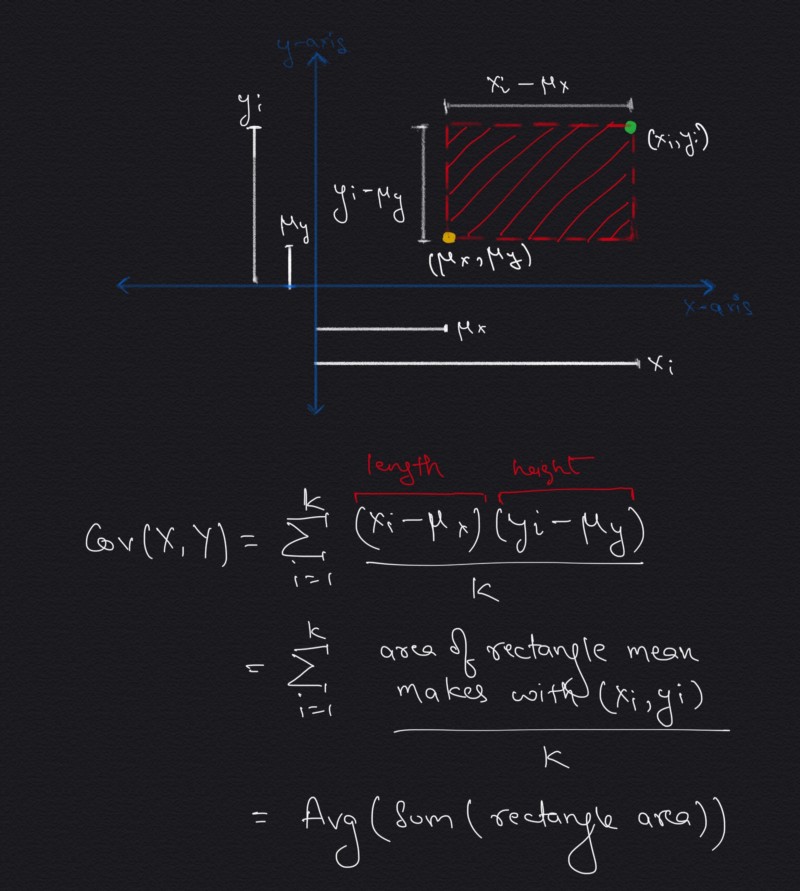 co-variance is nothing but average sum of all rectangle areas
So, it’s basically representing the area of a rectangle which is plotted between the mean and a data point. So each point of the dataset will make a rectangle with mean point. But as we draw rectangles for the complete dataset and find their area using the above formulae, we observe some rectangles have negative area! Nothing to worry, as it just showcase that this data point (for which we get -ve area) has different behavior for its variables, i.e. one is high but the other is low, which goes against the idea of co-variance. Now as we take the summation of all the data points’s rectangle area, what we are doing is adding the +ve areas and subtracting the -ve areas. And finally the resulting value after averaging represents the magnitude of co-variance. One examples on a sample dataset is shown below, where we showcase different points of dataset and the rectangles formed with their areas,
 Rectangles formed by the mean-point with rest of the points.
Negative area is represented as red, positive area by green.Let’s also look at the different datasets and the rectangles formed. Also notice that the Figure 1 represents the case with largest area and hence largest co-variance (we discussed how they are proportional). As stated before, the behavior shown here is the ideal one i.e. as one variable increases, so does the other. And as points starts to deviate from this straight line behavior, as shown in the subsequent figures, the amount of red rectangles increases and hence the magnitude of co-variances decreases.
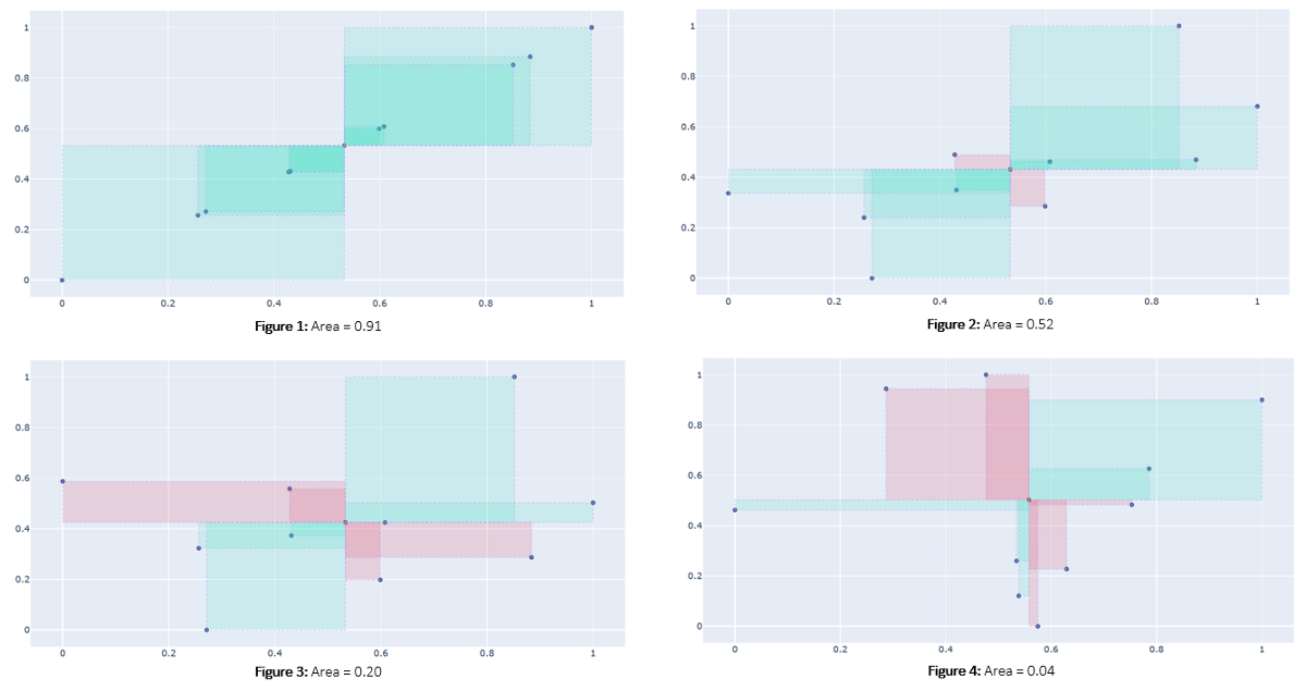
A decrease in area from figure 1 to figure 4, due to change in expectation of “both variables should show similar behavior”
Conclusion
When we represent a formula in an easily interpretable form such as a diagram or plot, it becomes much easier to understand and also easier to grasp hidden insights. For example if we represent co-variance in form of rectangles and their areas, we can quickly answer questions like which will have higher co-variance, an exponential decay or growth plot? Or what will happen if there are many +ve points near mean but one -ve point far away from the mean? (read, outliers). Try to think of these questions in the form of rectangles and areas and the answer will come out quickly. I hope it does :)
Reference
[1] https://en.wikipedia.org/wiki/Expected_value
[2] https://en.wikipedia.org/wiki/Standard_deviation
[3] https://en.wikipedia.org/wiki/Variance
[4] https://en.wikipedia.org/wiki/Covariance
For any question, feel free to connect with me on linkedin or visit more articles like this on my website.
Cheers.