Introduction to Acoustic event detection technique
Accurately identifying the occurrence of acoustic signatures, like birds chipping, human speaking, etc., from large audio files.

Introduction
Big data provides multiple applications, provided we clear the first and maybe the biggest hurdle of all, identifying interesting patterns or even segregating the meaningful parts from the junk. Ecologist are facing the same problem, with access to hours of recording of forest with all of its elements in its entirety, how can we separate out the important ones, like the sound of a tiger approaching or birds chipping. This calls for an intelligent technique to separate out the garbage which may include background noise of forest like sound of wind blowing, leaves rustling or event distant traffic (in current context). By removing all these, we may able to identify the interesting parts, which categories as acoustic events.
Step 1: Signal Pre-processing
First, lets get the data in a generic format. To start with, we can down sample the data to 22,050 Hz and with 16 bit depth. This means for 1 second of audio data, we have ~22 thousand samples, where each sample can have around 2¹⁶ (65,536) level of samplings or resolution.
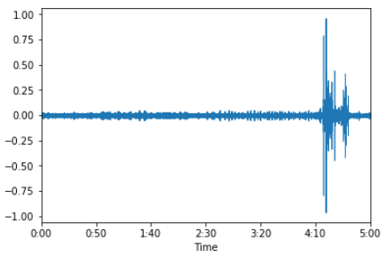
Audio waveform for a duration of 5 mins. X-axis is time, Y-axis is amplitude.Now instead of performing further analysis on this modified waveform, which deals with only 2-dimensions, i.e. time and amplitude, lets transform the data into 3-dimensions by including frequency as well. We can do that by generating spectrogram of the audio waveform. To do so we need to first create frames of 512 samples with 50% overlap, over which Hamming window is applied. After this we pass each frame to a FFT (Fast Fourier Transform) function and get in return amplitude values for 256 frequency bins. To smooth out the results, we apply a moving average of width 3. Finally the amplitude values are converted to decibels by applying following function,
Amplitude to decibels. Now, instead of performing all these steps, we can make use of matplotlib python library, and the conversion becomes as easy as,
>> import matplotlib.pyplot as plt
>> import numpy as np
>> _, freqs, t, im = \
plt.specgram(x = indata[0], Fs = indata[1], window = np.hamming(512), NFFT = 512, noverlap = 256)
Here, indata[0] is the array of waveform amplitude, indata[1] contains the sampling frequency (here, 22050). window signifies the smoothing window applied and its size, here its hamming of size equal to that of each frame i.e. 512. NFFT is each frame’s size and noverlap is sample size of overlapping, as 50% of 512 is 256. After this our waveform transforms into,
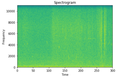
Spectrogram with time on X-axis, frequency on Y-axis and decibel amplitude as intensity of image.
Step 2: Wiener Filtering
Before going further, we need to smooth up the edges in the generated spectrogram. This will be help with removal of background graininess and blurring of acoustic events. This also helps by reducing the number of very small distributed events getting generated in the final output. For this we can use a 5x5 Wiener 2-d matrix and apply it to the spectrogram.
>> from scipy.signal import wiener
>> im = wiener(im, (5, 5))
The output look like a blurred images of the original image,
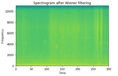
After applying the 5x5 Wiener filter.
Step 3: Noise reduction
To better assess the acoustic events we need to handle the noise which gets generated along with the events, specially those which are spread across the frequency domain. The contribution of noise to recordings of the environment data declines with increase in frequency. For this modified adaptive level equalization is applied. For each row of the spectrogram image, a histogram of the decibel intensity value is computed, where the bin width is 1 dB. After smoothing the histogram, we determine the modal noise intensity, which is located at the maximum bin in the lower half of the histogram.
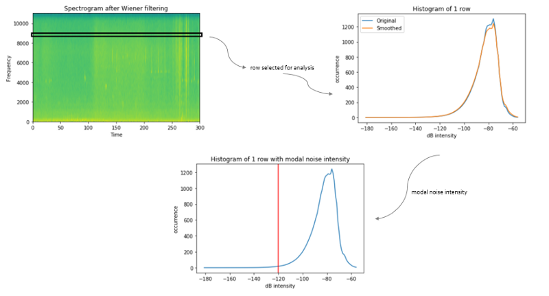
Iterative procedure to be repeated for each row of the spectrogram image.After repeating the same procedure for all rows, we get the modal noise intensity for the complete duration. Now we smooth this intensity vector to eliminate unwanted banding in the noise reduced spectrograms.
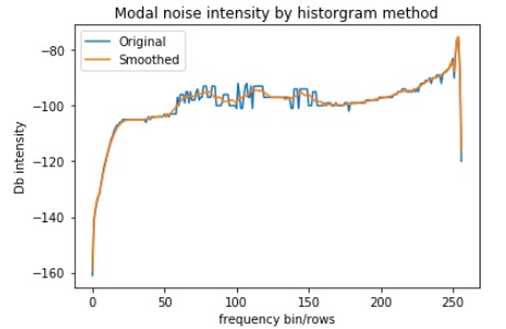
Modal intensity for the sonogram, with and without smoothing applied.Finally we remove the individual noise intensity from the spectrogram and clip every negative value to zero. This provide us with a noise removed image of the original spectrogram.
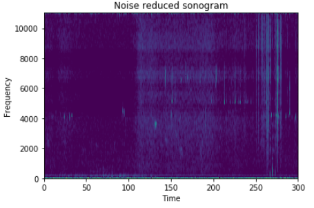
From complete greenish to highly minimal colored. Excessive noise has been removed.
Step 4: Binary conversion
As our final goal is to find valid events, any potential event can hold only two possible states, either its an event or its not. Hence, we need to convert our image into a binary image which showcase the binary presence of an event. This can be done by setting a single intensity threshold and any value more than that is an event, and any value below is background noise. This threshold is user and application dependent, but for most cases value between 6–9 dB will do. In our case, lets select the value to be 6 dB and convert the image to binary based on our discussed logic.
>> binary_threshold = 6
>> im_bw = np.array([x[:] for x in im])
>> im_bw[np.where(im > binary_threshold)] = 1
>> im_bw[np.where(im <= binary_threshold)] = 0
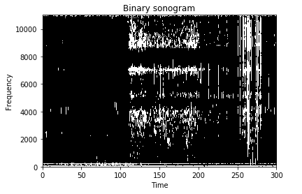
Color image transformed to black and white. White signifies event.Here, black is background and white is an event signature.
Step 5: Rejoining broken events
An event is spread across time and frequency dimension, and is distinguished by finding the continuous spread in these dimensions. In simple terms, a single blob of white in the binary sonogram is one event. Multiple events will be separated by black patches between them. But due to the single threshold value binary conversion in last step, a single low intensity event may breakup into multiple smaller intensity events. To handle this, we need to identify and rejoin such events to form a single event. We do this by joining event that are separated from each other by N or fewer pixels in vertical or horizontal directions. By default we can select N to be 1. So if two white blobs has a black single pixel patch between them, we fill up the black patch to join the two events.
Step 6: Identify acoustic events
Now we need to identify individual events, which can be handled by image processing. In the binary sonogram image, we need to identify the boundaries of separated out white patches. This make this a contour or boundary finding problem. Using the CV2 python image processing library which has a very efficient contour finding implementation, all we need is to pass the image and get a list to contours (here events) as output.
>> _, contours, _ = cv2.findContours(im, cv2.RETR_TREE, cv2.CHAIN_APPROX_NONE)
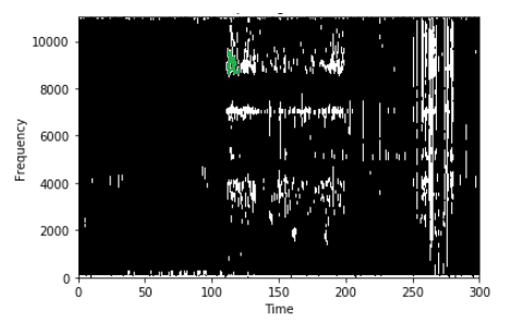
One of the detected events shaded with green.
Step 7: Removal of small events
Even after all the preliminary steps to remove unwanted events, there is always a possibility of some unexplained or unwanted event which bypassed previous steps. To handle this, we will perform a final post-processing of the detected events in this last step. Note, for each contour or events detected, as they are nothing but a blob or patch in a 2d image, we can associate area to them. So each event has some area, which is nothing but the area of the white blob. All we want to say is, if an event’s area is less than some threshold, its noise, otherwise its a valid one. Instead of blindly trusting the user’s threshold, we can apply the image distribution analysis to automatically verify the threshold. To do so, lets say we have a user threshold of 200 ( p_small ), i.e. as per the user any event with area less than 200 is noise, we will identify all events with area less than 200 and form a 10-bin histogram. The verified threshold is the first minimum from the left-hand side of the histogram. Any event with area less than this identified threshold is removed and the remaining (including the ones with area more than p_small are the identified events).
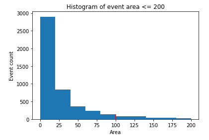
The first left-hand side minimum is 200 i.e. the last bin.From here, we can see the verified threshold is also 200, it seems the user was correct all along. But in most cases this may not be true and it doesn’t cost much to verify it. Hence here we choose the correct threshold as 200 and remove all events with area less than this.
Conclusion
For each detected events, we can identify its time of start (left most pixel’s co-ordinate of the respective white blob), its duration (the spread of blob in the x-axis) and also its high and low frequency (top and bottom most pixel’s co-ordinate of the blob in y-axis). In the end, the input of an audio file is transformed into a table of detected events along with their basic information. The two variable of interaction are binary_threshold and p_small which user can increase and/or decrease as per the application and required output to get varied result.
References
[1] Acoustic analysis of the natural environment, Michael Towsey and Birgit Planitz
For more such articles please visit my personal blog.
Cheers.