Introduction to Graph Neural Networks with DeepWalk

Introduction
Graph Neural Networks are the current hot topic [1]. And this interest is surely justified as GNNs are all about latent representation of the graph in vector space. Representing an entity as a vector is nothing new. There are many examples like word2vec and Gloves embeddings in NLP which transforms a word into a vector. What makes such representation powerful are (1) these vectors incorporate a notion of similarity among them i.e. two words who are similar to each other tend to be closer in the vector space (dot product is large), and (2) they have application in diverse downstream problems like classification, clustering, etc. This is what makes GNN interesting, as while there are many solutions to embed a word or image as a vector, GNN laid the foundation to do so for graphs. In this post, we will discuss one of the initial and basic approaches to do so - DeepWalk [2]
Graphs 101
Graph or Networks is used to represent relational data, where the main entities are called nodes. A relationship between nodes is represented by edges. A graph can be made complex by adding multiple types of nodes, edges, direction to edges, or even weights to edges.
![Figure 1: Karate dataset visualization @ Network repository [3].](/img/deep_walk_post/Untitled.png)
One example of a graph is shown in Figure 1. The graph is the Karate dataset [4] which represents the social information of the members of a university karate club. Each node represents a member of the club, and each edge represents a tie between two members of the club. The left info bar states several graph properties like a number of nodes, edges, density, degree, etc. Network repository [3] contains many such networks from different fields and domains and provides visualization tools and basic stats as shown above.
Notion of similar nodes
As the idea behind vector embedding is to highlight similarities, we will consider some definitions for similar nodes. Two nodes can be called similar by several ways, like if they have a similar — in-degree count, out-degree count, avg-degree, or no of neighbors, etc. One interesting notion is to consider the neighbors of nodes and the more common neighbors they share, more similar they are. In plain text, a node is defined by the company it keeps. If two nodes have very similar company, they are very similar. This idea of representing an entity by its locality is not new. The base of word embedding in NLP is based on the motto that, “a word is represented by the context it keeps”. With this much similarity between the two fields, its obvious that the first instinct was to leverage the existing techniques in NLP, port it to graph domains by somehow converting the idea of context of words to neighbor of nodes. One such existing technique is word2vec, which we will discuss briefly.
Word2Vec
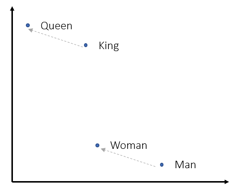
A detour with word2vec (w2v) is required to completely appreciate and understand the idea behind DeepWalk. Word2Vec is a word embedding technique that represents a word as a vector. Each vector can be thought of as a point in $R^{D}$ space, where $D$ is the dimension of each vector. One thing to note is that these vectors are not randomly spread out in the vector space. They follow certain properties such that, words who are similar like cat and tiger are relatively closer to each other than a completely unrelated word like tank. In the vector space, this means their cosine similarity score is higher. Along with this, we can even observe famous analogies like king - man + woman = queen which can be replicated by vector addition of these word’s representation vector.
While such representation is not unique to w2v, its major contribution was to provide a simple and faster neural network based word embedder. To do so, w2v transformed the training as a classification problem where given one word the networks try to answer which word is most probable to be found in the context of the given word. This technique is formally called Skip-gram, where input is the middle word and output is context word. This is done by creating a 1-layer deep neural network where the input word is fed in one-hot encoded format and output is softmax with ideally large value to context word.
![Figure 3: SkipGram architecture (taken from Lil'Log [7]). Its a 1 layer deep NN with input and output as one-hot encoded. The input-to-hidden weight matrix contains the word embeddings.](/img/deep_walk_post/Untitled 2.png)
The training data is prepared by sliding a window (of some window size) across the corpus of large text (which could be articles or novels or even complete Wikipedia), and for each such window the middle word is the input word and the remaining words in the context are output words. For each input word in vector space, we want the context words to be close but the remaining words far. And if two input words will have similar context words, their vector will also be close. This is the intuition behind Word2Vec which it does by using negative sampling. After training we can observe something interesting - the weights between the Input-Hidden layer of NN now represent the notions we wanted in our word embeddings, such that words with the same context have similar values across vector dimension. And these weights are used as word embeddings.
![Figure 4: Heatmap visualization of 5D word embeddings from Wevi [5]. Color denotes the value of cells.](/img/deep_walk_post/Untitled 3.png)
The result in Figure 4 is from training 5D word embeddings from a cool interactive w2v demo Wevi [5]. As obvious words like (juice, milk, water) and (orange, apple) have similar kinds of vectors (some dimensions are equally lit - red or blue). Interested readers can go to [7] for a detailed understanding of the architecture and maths. Also [5] is suggested for excellent visualization of the engine behind word2vec.
DeepWalk
DeepWalk employs the same training technique as of w2v i.e. skip-gram. But one important thing remaining is to create training data that captures the notion of context in graphs. This is done by random walk technique, where we start from one node and randomly go to one of its neighbors. We repeat this process $L$ time which is the length of the random walk. After this, we restart the process again. If we do this for all nodes (and $M$ times for each node) we have in some sense transformed the graph structure into a text like corpus used to train w2v where each word is a node and its context defines its neighbor.
Implementation 1: Author’s code
The DeepWalk authors provide a python implementation here. Installation details with other pre-requisite are provided in the readme (windows user be vary of some installation and execution issues). The CLI API exposes several algorithmic and optimization parameters like,
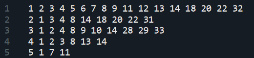
inputrequires the path of the input file which contains graph information. A graph can be stored in several formats, some of the famous (and supported by the code) are — adjacency list (node-all_neighbors list) and edge list (node-node pair which have an edge).number-walksThe number of random walks taken for each node.representation-sizethe dimension of final embedding of each node. Also the size of hidden layer in the skipgram model.walk-lengththe length of each random walk.window-sizethe context window size in the skipgram training.workersoptimization parameter defining number of independent process to spawn for the training.outputthe path to output embedding file.
Authors have also provided example graphs, one of which is our Karate club dataset. Its stored in the format of the adjacency list.
Now let’s read the graph data and create node embeddings by,
deepwalk --input example_graphs/karate.adjlist --number-walks 10
--representation-size 64 --walk-length 40 --window-size 5
--workers 8 --output trained_model/karate.embeddings
This performs start-to-end analysis by taking care of – loading the graph from the file, generating random walks, and finally training skip-gram model on the walk data. By running this with additional --max-memory-data-size 0 param, the script also stores the walk data as shown below.

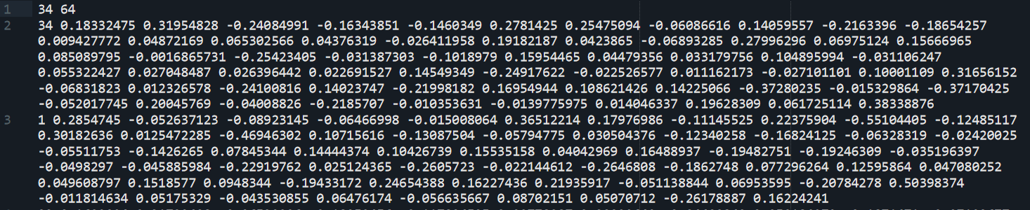
Finally, we get the output embedding file which contains vector embedding for each node in the graph. The file looks as,
Implementation 2: Karate club
A much simpler API is provided by newly released python implementation - KarateClub [6]. To do the same set of actions, all we need to do is following.
# import
import networkx as nx
from karateclub import DeepWalk
# load the karate club dataset
G = nx.karate_club_graph()
# load the DeepWalk model and set parameters
dw = DeepWalk(dimensions=64)
# fit the model
dw.fit(G)
# extract embeddings
embedding = dw.get_embedding()
The DeepWalk class also extends the same parameters exposed by the author’s code and can be tweaked to do the desired experiment.
![Figure 8: Parameters exposed by DeepWalk implementation in KarateClub [6].](/img/deep_walk_post/Untitled 7.png)
Experimentation
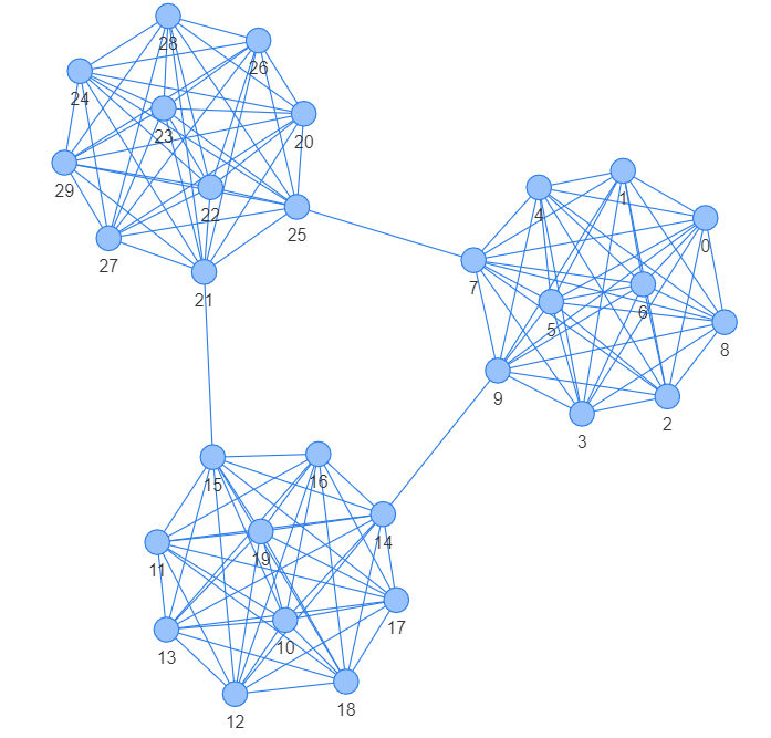
To see DeepWalk in action, we will pick one graph and visualize the network as well as the final embeddings. For better understanding, I created a union of 3 complete graphs with some additional edges to connect each graph.
Now, we will create DeepWalk embeddings of the graph. For this, we can use the KarateClub package and by running DeepWalk on default settings we get embeddings of 128 dimensions. To visualize this I use dimensionality reduction technique PCA, which scaled-down embeddings from $R^{128}$ to $R^2$. I will also plot the 128D heatmap of the embedding on the side.
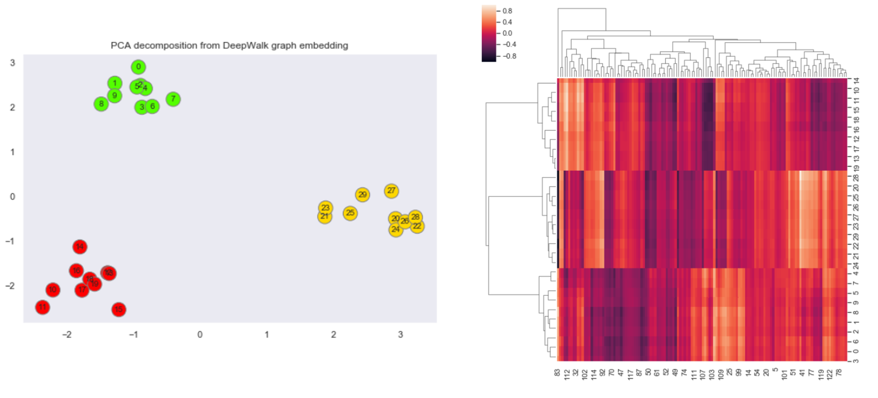
There is a clear segregation of nodes in the left chart which denotes the vector space of the embedding. This showcase how DeepWalk can transform a graph from force layout visualization to vector space visualization while maintaining some of the structural properties. The heatmap plot also hints to a clear segregation of graph into 3 clusters.
Another important thing to note is when the graph is not so complex, we can get by with lower dimension embedding as well. This not only reduces the dimensions but also improves the optimization and convergence as there are fewer parameters in skip-gram to train. To prove this we will create embedding of only size 2. This can be done by setting the parameter in DeepWalk object dw = DeepWalk(dimensions=2) . We will again visualize the same plots.
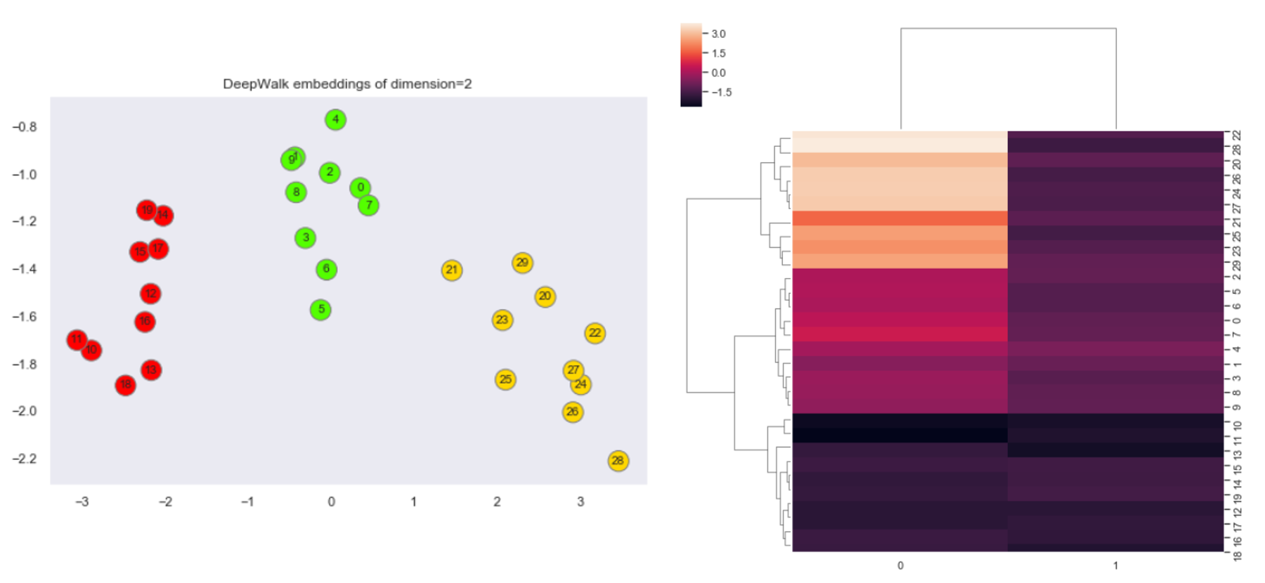
Both the plots again hint towards the same number of clusters in the graph, and all this by only using 1% of the previous dimensions (from 128 to 2 i.e. ~1%).
Conclusion
As the answer to this analogy NLP - word2vec + GraphNeuralNetworks = ? can arguably be DeepWalk (is it? 🙂 ), it leads to two interesting points, (1) DeepWalk’s impact in GNN can be analogous to Word2Vec’s in NLP. And it’s true as DeepWalk was one of the first approaches to use NN for node embeddings. It was also a cool example of how some proven SOTA technique from another domain (here, NLP) can be ported to and applied in a completely different domain (here, graphs). This leads to the second point, (2) As DeepWalk was published a while ago (in 2014 - only 6 years but a lifetime in AI research), currently, there are lots of other techniques which can be applied to do the job in a better way like Node2Vec or even Graph convolution networks like GraphSAGE, etc. That said, as to start with NN based NLP, word2vec is the best starting point, I think DeepWalk is in the same sense a good beginning for NN based graph analysis. And hence the topic of this article.
Cheers.
References
[1] EasyAI - GNN may be the future of AI
[4] Zachary karate club - The KONECT Project
[5] Wevi - word embedding visual inspector
[6] Karate club - Paper , Code
[7] Lil’Log - Learning word embedding