Introduction to Multi-dimensional Dynamic Programming
Understand the intuition behind the technique which solves miniature dependent problems to finally explain the problem in question.

What is dynamic programming?
It’s a technique to solve a special type of problems, which can be broken down into many dependent sub-problems. By dependent, I mean to solve one sub-problem you need the answer of other sub-problems. This differentiate dynamic programming (dp) from other methods like divide and conquer, where we usually create independent sub-problems. One of the most intuitive explanation of dp defines its as a directed graph, where nodes are the sub-problems and the edges between two nodes denotes the dependency of one problem on another.
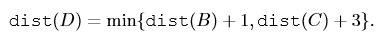
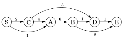 Fig 1: A directed graph with nodes being sub-problems and edges are dependency.To give one examples, we have to find the shorted path possible from S to D (consult Fig 1). Look closely, you can traverse to D via B or C, hence logically the shortest path should go through one of them. To formulate this, lets define dist(x) = shortest distance from S to any node ‘x’. We have to solve for dist(D), which can also be written as,
 Shortest path to D is function of Shortest path to B and C.In the same manner, dist(B) can be written in terms of A and dist(C) in terms of S. By solving each one of them, we get dist(D) i.e. the intended solution. To summarize, we are looking for problems which can be broken down in dependent sub-problems and they become candidate for dp application.
Possible approaches
Broadly there are two ways to solve dp problems,
- Top-down approach: In this we apply recursive technique to drill down to all dependent sub-problems required to solve the main problem. Here we start with the top i.e. the final problem, but to find it we must solve all sub-problems hence go down to solve them all. After combining them all, we have the final solution. For example in the last section, we started with dist(D) i.e. the main problem, and solved dist(B), dist(C), dist(A), etc to find it.
- Bottom-up approach: Here we begin from the base case i.e. the lowest possible sub-problem, iterate forward till we hit the final problem. For example, if we had started from S then traversed to C, A and then further up till we hit D, it would have been bottom-up approach.
Whats up with the dimensions?
We defined sub-problems and their dependency, other important entities in dp are the dependent elements or variables. The count of these variables defines the dimension of the problem. If a problem is dependent on 1 variable, its a 1D dp problem, similarly in case of 2 variables its 2D dp problem. Lets go through examples for each,
1-dimension DP problem
Suppose we want to find the fibonacci number at a particular index of the sequence. So fib(n) = nth element in the fibonacci sequence. So how should we go ahead and solve it using dp? Lets first try to identify sub-problems, is there any dependence of fib(n) with any of the predecessors like fib(n-1), fib(n-2)…fib(0)? Well of course, as per the definition, fib(n) = fib(n-1) + fib(n-2). And same goes on for fib(n-1) and fib(n-2) until we hit the base cases of fib(0) = 0 or fib(1) = 1. To formulate,
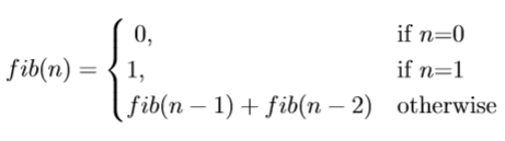 Fibonacci recursive formulaAs evident, we are using a top-down approach (we can also use bottom-up) and the dependent variable is only 1 i.e. ‘n’ which is the index number. Using this we can solve the fibonacci problem. Lets code it up,
One important point before moving on, a basic issue with recursive approach is it solves same problem multiples times. In our case, on plotting the function call in case of n = 5, we get
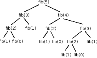 Recursive function calls for fib(5)Here, we want to solve for fib(5) which is called once, but other sub-problems have varied calls like fib(4) — 1, fib(3) — 2, fib(2) — 3, fib(1) — 5, fib(0) — 3. Its quite unintuitive to solve a same problems multiple times and we can handle it if we store the solution of a problem and next time when its called just pass the stored answer. This is called memoization. Modifying the previous code to be more optimal,
2-dimension DP problem
This type of problems have two dependent variables. Lets take a example of edit distance. In this problem, we are given two strings and we have to find a measure of dissimilarity between the two strings. This is calculated by placing (visually) one string on top of another and trying to find the best point of fit so that by applying minimum edits we can transform one string to another. Hence the name edit distance. The supported edits are insertion, deletion and substitution. As one of the main task requires finding the best point of fit, same pair of strings with different alignment or fit will give different edit distance. For example,
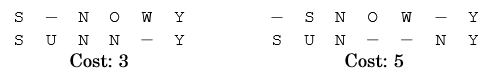 two different alignments with different costsConsider ‘snowy’ and ‘sunny’, above figure shows two possible fits. Now, how is the cost or edit distance is calculated? Take the left alignment, we need to perform 3 edits (hence the cost = 3) to transform snowy to sunny which are, (1) insert U at index 1, (2) substitute O with N at index 3, and (3) delete W at index 4.
Now, lets see if we can apply dp to solve this problem, for that we need to identify the dependent sub-problems. Our main problem is to find edit distance between two strings x[1..m] (of length m) and y1…n. What if we try to solve the problem for some prefix of x i.e. x[1…i] and y i.e. y[1…j]? Can we build upon this to solve the next problem? Take the previous example, if we know the edit distance for ‘sno’ and ‘sun’, can we use this to solve for ‘snow’ and ‘sunn’? Taking the last character of these strings i.e. ‘w’ and ’n’, formally we can perform only three operations,(1) either delete ‘w’ (2) insert ’n’, or (3) match ‘o’ with ‘w’ in which case they can be same or different (which leads to substitution), here they are different. In general we can perform these operations on any pair of x[i] and y[j]. In case of (1) we delete x[i] and we have to solve for the remaining x[1…i-1] and y[1…j] , for (2) we insert y[i], and we solve for x[1…i] and y[1…j-1] or (3) we solve for x[1…i-1] and y[1…j-1]. Nice! In all these cases, we just have to solve for smaller problem and keep adding the cost of possible edit operations, lets keep them all equal to 1 for now. Our formulae now becomes,
 edit distance where diff(i, j) = 0 if x[i] = y[j], otherwise 1As the problem is of 2 dimension — index of each strings — we need to maintain a 2d table to store all processed edit distances.
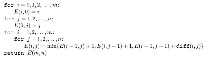
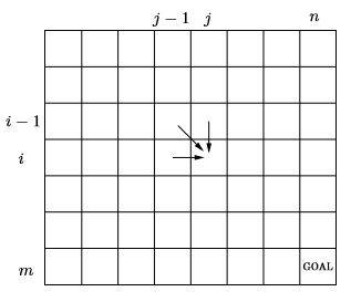 columns are for string 2 of size n, rows are for string 1 of size mHere, a cell (i, j) defines the edit distance required to transform string_1 till index i to string_2 till index j. With this our goal is to find the value at cell (m, n). Also as the edit distance at (i, j) requires value of 3 different cells, we need to traverse through the table in such a way that when we are at (i, j) we have already solved for (i-1, j), (i, j-1) and (i-1, j-1). Finally defining the base case, when either i =0 or j =0, so (0, 5) means to transform a blank string to 5 length string, which is simply 5 insertions hence cost is 5, same for (5,0). To factor this we add additional column and row in the table with these default values. Hence the pseudo code is,
 Lets code it up,
Solving the problem for ‘exponential’ and ‘polynomial’, our table transforms to,
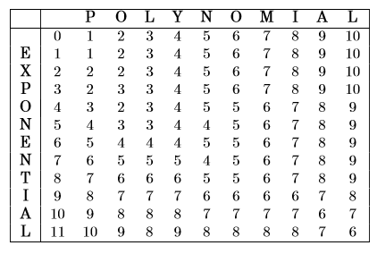 So the final edit distance between the two strings is 6.
Conclusion
We just touched the surface of the technique and tried to solve some classic problems. The most important and possibly the hardest part in dp is to correctly identify sub-problems, this process sometimes takes lots of exterminations. The idea behind the post was to provide readers with a brief introduction and intuition behind the logic of identifying dimensions and sub-problems. Once done, we have mostly solved the problem, all that’s left is to combine the sub-problems together into a nice formulation and rest falls into pieces perfectly. ss
Reference
[1] Algorithms, Book by Christos Papadimitriou, Sanjoy Dasgupta, and Umesh Vazirani
Please clap and share if you like the post and comment in case of any question. Also visit my **personal blog* for more such posts.*
Cheers.