Reinforcement Learning with Multi Arm Bandit (Part 2)

06 May 2018 - 7 mins read time
Tags: reinforcement-learning math python

This is Part 2 of two part articles. The combined article is present in the Lazy Data Science Guide.

Let make the problem a little bit more….complex!

Recap

This is in continuation of the original post, I highly recommend to go through it first, where we understood the intuition of multi arm bandit and tried to apply e-greedy algorithms to solve a representative problem. But the world isn’t that simple. There are some factors, introducing which, the problem changes completely and the solution has to be redefined. We will pick where we left, introduce new problem, show how our beloved algorithm fails and try to build intuition of what might help in the case.

Non-stationary problems

Previously, we had defined some portals with fixed reward distribution and tried to bring our estimated action value closer to the expected action value or reward distribution. For non-stationary problems, the bulk of the definitions remains same, but we will just tweak the part of fixed reward distribution. In the original problem, we defined a reward distribution function whose values were not changing throughout the process, but what if they are? What if expected action value is not constant? In terms of the Home portal game, what if the home portal is slowly becoming an ocean one or vice versa or just fluctuating at the border line? In such cases, will our simple e-greedy algorithm work? Well, lets try to find out.
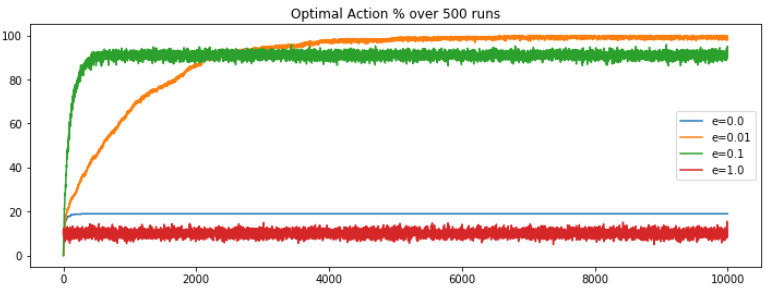
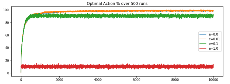
First, let’s re-run the original code for 10k steps and plot the optimal action selection percentage, the observation is nearly as expected. The epsilon value of 0.01 is out-performing the contrasting e = 0 or 1 but e = 0.01 is overtakes the other approaches around the 2k steps mark. Overtime the performance saturates, with no sign of decrease in the future.

Now, we need a slight modification to transform the stationary problem to non-stationary. As per the definition, the reward distribution is subject to change. Lets define the term of change, say after each step, and by a normal distribution with mean = 0 and deviation = 0.01. So after each step, we will compute random numbers based on the defined normal distribution and add it to the previous expected action value. This will become the new reward distribution. This could be easily done adding few lines to the original code, and then we can compute the latest optimal action selection percentage.

# define a function to update the expected_action_value  
def update_expected_action_value(expected_action_value, arms):  
    expected_action_value += np.random.normal(0, 0.01, arms)   
    return(expected_action_value)
    
# inside the multi_arm_bandit_problem function add,   
estimate_action_value = update_estimate_action_value(estimate_action_value)

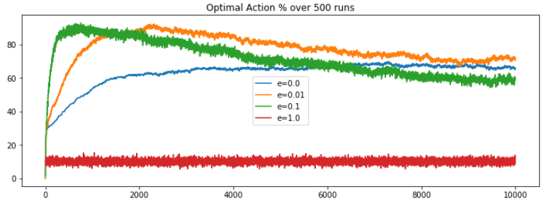
On comparing, we could say the performance of the e-greedy algorithms started decreasing after a certain period. Note, even though e=0.01 is still showing good results, but this drastic decrease in performance is visible even by a slight random increment (deviation=0.01), what if the change factor was of higher magnitude? Well as it turn out the decrease would have been more prominent. What is the problem here?

Formulation

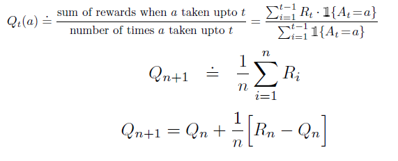
Try to recall the estimation function of the true reward distribution for stationary problem, it goes something like this,

where,

The first equation gives the formula for the estimated reward value for an action at t which is a simple average of all the rewards we received for that action till time t-1
The second equation is just a nice way of writing the same thing. It implies that the estimation of the reward for n+1 step will be average of all the rewards till step n
The third equation is what you get when you expand the second equation and put in the formulae of $Q_n$ which is similar to the one of $Q_{n+1}$, just one step less (replace n with n-1). Here, $Q_{n+1}$ is the new estimation for the n+1 steps, $Q_n$ is the old estimation i.e. estimation till step n, $R_n$ is the rewards for nth step and 1/n is step size by which we want to update the new estimation.

To be clear, as per this formulation, if a particular action was chosen say 5 times, then each of the 5 rewards (n actions leads to n rewards) will be divide by 1/5 and then added to get the estimation till step 5. If you look closer, you will see we are giving equal weights to all the rewards, irrespective of their time of occurrence, which means we want to say, every reward is equally important to us and hence the equal weights. This holds true for the stationary problems but what about the newer problem? With rewards distribution changing, isn’t the latest rewards better estimation of the true rewards distribution. So shouldn’t we just give more weight to the newer rewards and lesser to the old one?

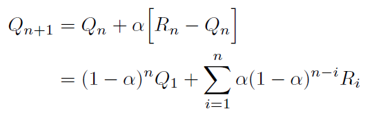
Well this thought is definitely worth pursuing. And this would mean just changing the reward weights, which can be done by replacing the average reward estimation to exponential recency-weighted average. We can further make this process generic by providing an option of if the newer or older rewards should be given more weight or a middle workaround of decreasing weights with time. As it turns out this could be easily done by replacing the step function of 1/n in the older formulation with a constant, say 𝛂. This updates the estimation function to,

where,

If 𝛂 = 1; $R_n$ i.e. the very latest reward will have maximum weight of 1 and rest will have 0. So if your excepted action value’s deviation is too drastic, we could use this setting.
If 𝛂 = 0; $Q_1$ i.e. the oldest reward estimation will have maximum weight of 1 and rest will have 0. We could use this when we only want to consider initial estimation values.
If 0 < 𝛂 < 1; the weight decreases exponentially according to the exponent 1-𝛂. In this case the oldest reward will have smaller weight and latest rewards higher. And this is what we want to try out.

The non-stationary solution

Lets formalize the solution by simply updating the code to replace the step size by an constant of value, say 0.1 and keeping rest of the parameters same. This will implement the exponential decreasing weight. Later we will compute the optimal action selection percentage and reflect on it.

# update the estimation calculation  
estimate_action_value[action] = \
    estimate_action_value[action] + \
    0.1 * (reward - estimate_action_value[action])

And we are back in business! e=0.01 is out-performing it’s rival and the performance converges to maximum after some steps. Here we are not seeing any decrease in performance, because of our modified estimation function which factor the changing nature of reward distribution.

Conclusion

The take away from this post could be understanding the stationary and non-stationary environment. The art of designing estimation functions by questioning and considering all the properties of the environment. And how sometimes minimal but intuitive changes could lead to maximum advancements in accuracy and performance. We still have some set of problems and improvements left which could lead to better accuracy and optimization, but later on that.

Cheers.

Reference

[1] Reinforcement Learning — An Introduction; Richard S. Sutton and Andrew G. Barto