String similarity — the basic know your algorithms guide!
A basic introduction to most famous and widely used, and still least understood algorithms for string similarity.
Introduction
What is the best string similarity algorithm? Well, it’s quite hard to answer this question, at least without knowing anything else, like what you require it for. And even after having a basic idea, it’s quite hard to pinpoint to a good algorithm without first trying them out on different datasets. It’s a trial and error process. To make this journey simpler, I have tried to list down and explain the workings of the most basic string similarity algorithms out there. Give them a try, it may be what you needed all along.
Types of algorithms
Based on the properties of operations, string similarity algorithms can be classified into a bunch of domains. Let’s discuss a few of them,
-
Edit distance based: Algorithms falling under this category try to compute the number of operations needed to transforms one string to another. More the number of operations, less is the similarity between the two strings. One point to note, in this case, every index character of the string is given equal importance.
-
Token-based: In this category, the expected input is a set of tokens, rather than complete strings. The idea is to find the similar tokens in both sets. More the number of common tokens, more is the similarity between the sets. A string can be transformed into sets by splitting using a delimiter. This way, we can transform a sentence into tokens of words or n-grams characters. Note, here tokens of different length have equal importance.
-
Sequence-based: Here, the similarity is a factor of common sub-strings between the two strings. The algorithms, try to find the longest sequence which is present in both strings, the more of these sequences found, higher is the similarity score. Note, here combination of characters of same length have equal importance.
Edit distance based algorithms
Let’s try to understand most widely used algorithms within this type,
Hamming distance
This distance is computed by overlaying one string over another and finding the places where the strings vary. Note, classical implementation was meant to handle strings of same length. Some implementations may bypass this by adding a padding at prefix or suffix. Nevertheless, the logic is to find the total number of places one string is different from the other. To showcase an examples,
>> import textdistance
>> textdistance.hamming('text', 'test')
1
>> textdistance.hamming.normalized_similarity('text', 'test')
0.75
>> textdistance.hamming('arrow', 'arow')
3
>> textdistance.hamming.normalized_similarity('arrow', 'arow')
0.4
As evident, in first example, the two strings vary only at the 3rd position, hence the edit distance is 1. In second example, even though we are only missing one ‘r’, the ‘row’ part is offset by 1, making the edit distance 3 (3rd, 4th and 5th position are dissimilar). One thing to note is the normalized similarity, this is nothing but a function to bound the edit distance between 0 and 1. This signifies, if the score is 0-two strings cannot be more dissimilar, on the other hand, a score of 1 is for a perfect match. So the strings in first example are 75% similar (expected) but in strings in second example are only 40% similar (can we do better?).
Levenshtein distance
This distance is computed by finding the number of edits which will transform one string to another. The transformations allowed are insertion — adding a new character, deletion — deleting a character and substitution — replace one character by another. By performing these three operations, the algorithm tries to modify first string to match the second one. In the end we get an edit distance.
>> textdistance.levenshtein('arrow', 'arow')
1
>> textdistance.levenshtein.normalized_similarity('arrow', 'arow')
0.8
As evident, if we insert one ‘r’ in string 2 i.e. ‘arow’, it becomes same as the string 1. Hence, the edit distance is 1. Similar with hamming distance, we can generate a bounded similarity score between 0 and 1. The similarity score is 80%, huge improvement over the last algorithm.
Jaro-Winkler
This algorithms gives high scores to two strings if, (1) they contain same characters, but within a certain distance from one another, and (2) the order of the matching characters is same. To be exact, the distance of finding similar character is 1 less than half of length of longest string. So if longest strings has length of 5, a character at the start of the string 1 must be found before or on ((5/2)–1) ~ 2nd position in the string 2 to be considered valid match. Because of this, the algorithm is directional and gives high score if matching is from the beginning of the strings. Some examples,
>> textdistance.jaro_winkler("mes", "messi")
0.86
>> textdistance.jaro_winkler("crate", "crat")
0.96
>> textdistance.jaro_winkler("crate", "atcr")
0.0
In the first case, as the strings were matching from the beginning, high score was provided. Similarly, in the second case, only one character was missing and that too at the end of the string 2, hence a very high score was given. Imagine the previous algorithms, the similarity would have been less, 80% to be exact. In third case, we re-arranged the last two character of string 2, by bringing them at front, which resulted in 0% similarity.
Token based algorithms
Algorithms falling under this category are more or less, set similarity algorithms, modified to work for the case of string tokens. Some of them are,
Jaccard index
Falling under the set similarity domain, the formulae is to find the number of common tokens and divide it by the total number of unique tokens. Its expressed in the mathematical terms by,
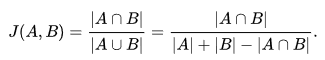
Jaccard index where, the numerator is the intersection (common tokens) and denominator is union (unique tokens). The second case is for when there is some overlap, for which we must remove the common terms as they would add up twice by combining all tokens of both strings. As the required input is tokens instead of complete strings, it falls to user to efficiently and intelligently tokenize his string, depending on the use case. Examples,
>> tokens_1 = "hello world".split()
>> tokens_2 = "world hello".split()
>> textdistance.jaccard(tokens_1 , tokens_2)
1.0
>> tokens_1 = "hello new world".split()
>> tokens_2 = "hello world".split()
>> textdistance.jaccard(tokens_1 , tokens_2)
0.666
We first tokenize the string by default space delimiter, to make words in the strings as tokens. Then we compute the similarity score. In first example, as both words are present in both the strings, the score is 1. Just imagine running an edit based algorithm in this case, the score will be very less if not 0.
Sorensen-Dice
Falling under set similarity, the logic is to find the common tokens, and divide it by the total number of tokens present by combining both sets. The formulae is,
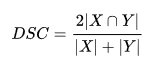
Sorensen-Dice formulaewhere, the numerator is twice the intersection of two sets/strings. The idea behind this is if a token is present in both strings, its total count is obviously twice the intersection (which removes duplicates). The denominator is simple combination of all tokens in both strings. Note, its quite different from the jaccard’s denominator, which was union of two strings. As the case with intersection, union too removes duplicates and this is avoided in dice algorithm. Because of this, dice will always overestimate the similarity between two strings. Some example,
>> tokens_1 = "hello world".split()
>> tokens_2 = "world hello".split()
>> textdistance.sorensen(tokens_1 , tokens_2)
1.0
>> tokens_1 = "hello new world".split()
>> tokens_2 = "hello world".split()
>> textdistance.sorensen(tokens_1 , tokens_2)
0.8
Sequence based algorithm
Lets understand one of the sequence based algorithms,
Ratcliff-Obershelp similarity
The idea is quite simple yet intuitive. Find the longest common substring from the two strings. Remove that part from both strings, and split at the same location. This breaks the strings into two parts, one left and another to the right of the found common substring. Now take the left part of both strings and call the function again to find the longest common substring. Do this too for the right part. This process is repeated recursively until the size of any broken part is less than a default value. Finally, a formulation similar to the above-mentioned dice is followed to compute the similarity score. The score is twice the number of characters found in common divided by the total number of characters in the two strings. Some examples,
>> string1, string2 = "i am going home", "gone home"
>> textdistance.ratcliff_obershelp(string1, string2)
0.66
>> string1, string2 = "helloworld", "worldhello"
>> textdistance.ratcliff_obershelp(string1, string2)
0.5
>> string1, string2 = "test", "text"
>> textdistance.ratcliff_obershelp(string1, string2)
0.75
>> string1, string2 = "mes", "simes"
>> textdistance.ratcliff_obershelp(string1, string2)
0.75
>> string1, string2 = "mes", "simes"
>> textdistance.ratcliff_obershelp(string1, string2)
0.75
>> string1, string2 = "arrow", "arow"
>> textdistance.ratcliff_obershelp(string1, string2)
0.88
In first example, it found ‘ home’ as the longest substring, then considered ‘i am going’ and ‘gone’ for further processing (left of common substring), where again it found ‘go’ as longest substring. Later on right of ‘go’ it also found ’n’ as the only common and longest substring. Overall the score was 2 * (5 + 2 + 1) / 24 ~ 0.66. In second case, it found ‘hello’ as the longest longest substring and nothing common on the left and right, hence score is 0.5. The rest of the examples showcase the advantage of using sequence algorithms for cases missed by edit distance based algorithms.
Conclusion
The selection of the string similarity algorithm depends on the use case. All of the above-mentioned algorithms, one way or another, try to find the common and non-common parts of the strings and factor them to generate the similarity score. And without complicating the procedure, majority of the use cases can be solved by using one of these algorithms. A little more complicated domains include vector representation and compression types, which also consider the semantic of the words or n-grams. More on this later.
References
[1] Levenshtein Distance, in Three Flavors — by Michael Gilleland, Merriam Park Software
[2] Hamming distance
[3] Jaro-Winkler
[4] Jaccard Index
[5] Dice coefficients
[6] Pattern matching — Gestalt approach (Ratcliff-Obershelp similarity)
[7] textdistance — python package
For more similar posts visit my personal blog.
Cheers.