Understanding the forecasting algorithm: STLF Model
Predicting the future based on historical information

Introduction
Lets start with understanding what is forecasting all about? Well its the best prediction of the future values provided the insights learned from the historical data. And as simple as it may sound, every forecasting algorithms tries to do so, alas with different assumptions. The STLF algorithm in question tried to forecast into the future, based on assuming the presence of different properties of a time series and how deeply embedded these properties are. Lets understand these properties.
STLF Model
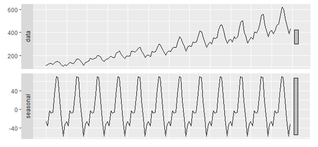
STLF can be defined as Seasonal and Trend decomposition using Loess Forecasting model. Well that’s mouthful. But the complete procedure could be divided into decomposition and forecasting, where one paves the way for another. STLF modeling assumes that a timeseries can be broken down in error, trend and seasonality components. So if finding patterns in original timeseries was difficult, the decomposition could make the process a little easier; and if we are able to replicate decomposed pattern for future, the forecasting is nothing but recombining the components. Lets understand each components and what they signify,
- **Trend: **A trend exists when there is a long-term increase or decrease in the data. It does not have to be linear.
- **Seasonality: **A seasonal pattern occurs when a time series is affected by seasonal factors such as the time of the year or the day of the week. Seasonality is always of a fixed and known frequency.
- Error: It is the random value remaining after we remove the trend and seasonality from the timeseries data. There should be no pattern in the error term, and if it is, well then we have done a lousy job in decomposing.
Decomposition
Now that we have a basic intuition of the components, lets understand the decomposition procedure. Throughout this post we consider the air passenger dataset which provided monthly passenger count from 1949 to 1960, it looks like this,
 Air Passenger monthly dataset for 11 yearsHm, there seems to be some pattern in the data. Lets try to decompose the timeseries, first starting with,
**Seasonality: **To be generic, if a dataset’s seasonality is composed ofx points (period) then the average seasonality could be computed by taking average of all the i + (i+x) + (i+2x) + … points. Lets see if our dataset has some seasonality or not. For that lets plot the data with each month separated out.
 Monthly plot for the air passenger dataset for every year.From the plot we can say, there seems to be some decline as we move from Jan to Feb, then as we move towards Jul there seems to be increase in the passenger count and from Aug we see a decline in count followed by another increase during Dec. And as this pattern is evident for a number of years, we can conclude our data has yearly seasonality. So in our case of monthly data for 11 years, seasonality could be computed by taking average of every years’s January, February and so on. Replicating the average data to cover the size of the data, we get this,
 Seasonal decomposition of the air passenger dataset**Trend: **The trend calculation is nothing but smoothing the data, which corresponds to representing a bucket of data points by a single point. This could help us identify the overall trend of the data. This could be achieved either by moving average (take weighted average of a bucket of data) or by loess smoothing (use local weighted regression to fit the points). As the definition of STLF suggest (L is Loess), we will prefer Loess smoothing here. Now the question is what should be the bucket size, for which the local regression will be done. One intuitive way is to keep it same as the length of the period of seasonality. This way we are negating the seasonality in the trend component; and any pattern in trend could relate to another insight for forecasting. For the air passenger dataset, as seasonality is yearly, the period will be 12 (#months in year). We will perform smoothing with this bucket size. The resulting trend looks like this,
 Trend computed by loess smoothing for air passenger dataset**Error: **This is what you get when you remove the trend and seasonality from the original dataset. So after computing rest of components, remove them from the dataset and viola the remaining presumed random values are error.
 Error component for the air passenger dataset#### Forecasting
Now that we have all the required components, lets think how we can use this knowledge for predicting the future values. Talking about seasonality, it is the pattern we have discovered in the data and as this pattern is repetitive for the last couple of years, we can assume same will happened for the next. So lets keep the seasonality as it is. Now for the remaining components, lets combine the trend & error and call this combination seasonally adjusted data (as it is original minus season, get it?). Now if we are able to do some prediction here, we will take care of the trend. As evident from the data, the trend is increasing throughout the data and say if we are able to predict future trend and combine it with the predicted seasonality (which is nothing but averaged last year’s seasonality) we have forecasted the air passenger dataset for unseen next year!
Now to predict the seasonally adjusted data there are bunch of options available from using the naive method to EST model to even ARIMA modelling. But to keep the post simple and as we haven’t talked about other forecasting model, lets use naive method here. Naive method suggests that forecast value is same as the last evident value.
 Air passenger’s seasonal adjusted data with naive forecastingNow when we combine this with the computed season data, we get the forecasted data for the air passenger, which looks like,
 Air Passenger data forecasting using naive methodConclusion
Not bad, as we were able to identify and replicate the seasonality but still there are some point that need focus. We can conclude the following from the plot,
- The trend is completely lost, the forecasted value is coming in straight.
- The seasonality is also constant, but it should be increasing as evident from the data. So what went wrong here? One word answer, the Naive method. STLF in general are quite basic but powerful forecasting technique. Just combine them with ETS and ARIMA for seasonally adjusted data prediction and you will get state-of-the-art forecasting for a large variety of data. Now what we used here is Naive method which has drawbacks like it is not able to model the trend which is evident from the forecasted plot, as now the future values look straight. Using any other combination with STL other than naive would have been out of scope but just to showcase the prowess of STL, lets see how they would have looked.
 Air passenger forecasting using ETS for seasonally adjusted data
 Air passenger forecasting using ARIMA for seasonally adjusted dataMaybe another post where we can discuss each of these method and why they outperform the naive method.
Reference
[1] Forecasting: Principles and Practice — Rob J Hyndman and George Athanasopoulos