LSTM, GRU and RNN
Introduction
- LSTM, GRU or RNN are a type of recurrent layers. They were the state-of-the-art neural network models for text related applications before the transformers based models. They can be used to process any sequential data like timeseries, text, audio, etc. RNN is the simpler of the lot, where as LSTM and GRU are the "gated" (and so a little complex) version of RNN. These gates helps LSTM and GRU to mitigate some of the problems of RNN like exploding gradient.
- The most basic unit in these layers is a "cell", which is repeated in a layer - equal to the number of token size. For example, if we want to process a text with 150 words (with word level tokenization), we need to perceptually attach 150 cells one after the another. Hence, each cell process one word and passes on the representation of the word (hidden state value) to the next cell in line.
- Starting with RNN, the flow of data and hidden state inside the RNN cell is shown below.
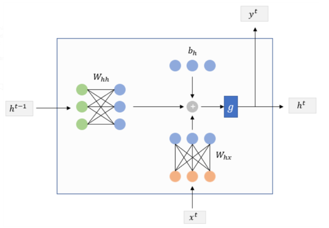
- As shown in the figure,
x^tis the input token at timet,h^{t-1}is the hidden state output from the last step,y^tandh^tare two notations for the hidden state output of timet. The formulation of an RNN cell is as follow,
\[
h^{t}=g\left(W_{h h} h^{t-1}+W_{h x} x^{t}+b_{h}\right) \\
y^{t}=h^{t}
\]
- LSTM cells on the other hand is more complicated and is shown below.
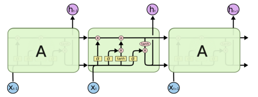
Note
Python libraries take liberty in modifying the architecture of the RNN and LSTM cells. For more details about how these cells are implemented in Keras, check out (practical_guide_to_rnn_and_lstm).
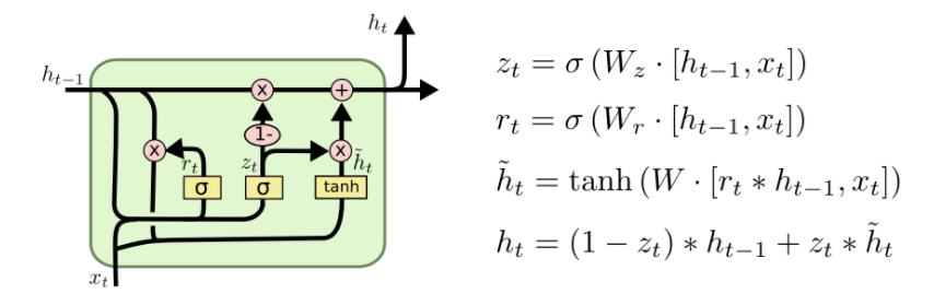
- Finally, a GRU cell looks as follow,
- While RNN is the most basic recurrent layer, LSTM and GRU are the de facto baseline for any text related application. There are lots of debate over which one is better, but the answer is usually fuzzy and it all comes down to the data and use case. In terms of tunable parameter size the order is as follow -
RNN < GRU < LSTM. That said, in terms of learing power the order is -RNN < GRU = LSTM. - Go for GRU if you want to reduce the tunable parameters but keep the learning power relatively similar. That said, do not forget to experiment wth LSTM, as it may suprise you once in a while.
Code
Using BiLSTM (for regression)
1 2 3 4 5 6 7 8 9 10 11 12 13 14 15 16 17 18 19 20 21 22 23 24 25 26 27 28 29 30 31 32 33 34 35 36 37 38 39 40 41 42 43 44 45 46 47 48 49 50 51 52 53 54 55 56 57 58 59 60 | |
Additional materials
- A practical guide to RNN and LSTM in Keras (practical_guide_to_rnn_and_lstm)
- Guide to Custom Recurrent Modeling in Keras (Guide_to_custom_recurrent_modeling)
- Understanding LSTM Networks (lstm_understanding)